
Now that we have gone through the tasks of downloading Jupyter and configuring it to our liking, we can start to work our way through the various tools it has to offer us. Before we get into anything too heavy, let us start out by renaming our Notebook to something a little more memorable. Your Notebook will probably be named something like ‘Untitled’ at the very top of your Notebook. To rename this, simply click on the name ‘Untitled’ and type in your preferred name. This will save automatically but if you want you can also just hit the save icon to do this manually. Jupyter autosaves every 120 seconds to a ‘checkpoint file’ which doesn’t alter your main primarily Notebook - this means that any crashes can be entirely recoverable. You can also revert to any given checkpoint by going ‘‘File > Revert to Checkpoint’’.
There are two really important terms we should know about prior to any actual coding in our Notebook. The first is a ‘kernel’, think of this as the entire block of the Notebook that deals with executing all the code that is contained in the document. The second is a ‘cell’, each cell is a container for text to be displayed in the notebook or for code to be executed by the notebook’s kernel. A Notebook will have one kernel that executes the code from many cells.
To break this down slightly more. A cell is the backbone of the Notebook. there are two main types of cells that you should know about. The first is a ‘code cell’ this is where our code goes to be executed by our kernel. When the code is executed, the notebook will display the output below the code cell that generated it. The second is a ‘Markdown cell’. This contains text formatted using Markdown and will be where you can add additional information that goes above and beyond simple comments in a .do file. To create a new cell in Notebook simply click on the plus icon next to the save icon on the top panel.
When running Stata in our Jupyter Notebook there is one golden rule to remember because each cell is separate from one another, each time we wish to execute some code within Stata, we have to call upon it prior to any code. As an example, say I wanted to use a specific dataset on my local disk drive, I would first have to add:
%%stata
Prior to adding within the same code cell:
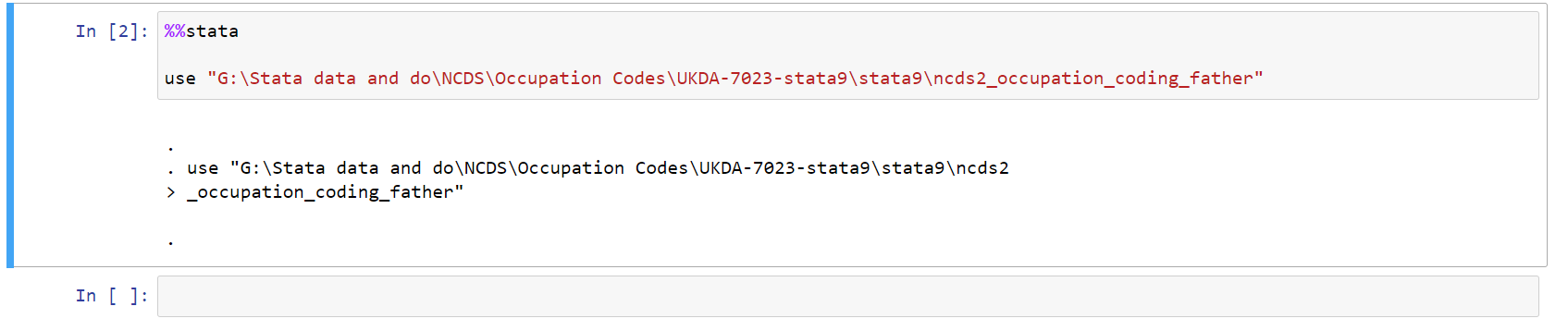
use "G:\Stata data and do\NCDS\Occupation Codes\UKDA-7023-stata9\stata9\ncds2_occupation_coding_father"
This may sound slightly tedious but remember, the reason we do this is because Jupyter Notebook allows us to use multiple programming languages at the same time across the same environment - I can theoretically clean my code up in Stata and then run my data visulisation in Python or R.
Prior to hitting the ‘Run’ button at the top of our Jupyter Notebook the code looks very similar to that of any .do file:

However, after we click ‘Run’, both the code and the output are produced on the same Notebook:
This doesn’t look so amazing with a simple ‘use’ command, but when we start introducing statistical models and visualisations into the mix, the attractiveness of using Jupyter Notebook becomes easier to understand.
Whilst we have so far displayed the code cell and its execution, when writing code - especially code that can be replicated, we also require detailed comments not just on the code itself but on the research process. For this, we use Markdown cells. Say I wanted to look at how Parental Social Class impacts youth employment trajectories. For this, I would need two things, a variable on parental social class and a set of variables on youth employment trajectories. Fortunately for me, the National Childhood Development Study has just the variables I require, though they are across datasets as this is longitudinal data. I’d need to merge the datasets and also rename the unique id as in some datasets it is capitalised, in others, it is not. If I were to simply do all of this without mentioning it, it would be extremely confusing for anyone trying to follow along with my code - if I provided my code at all. This is where Markdown shines:
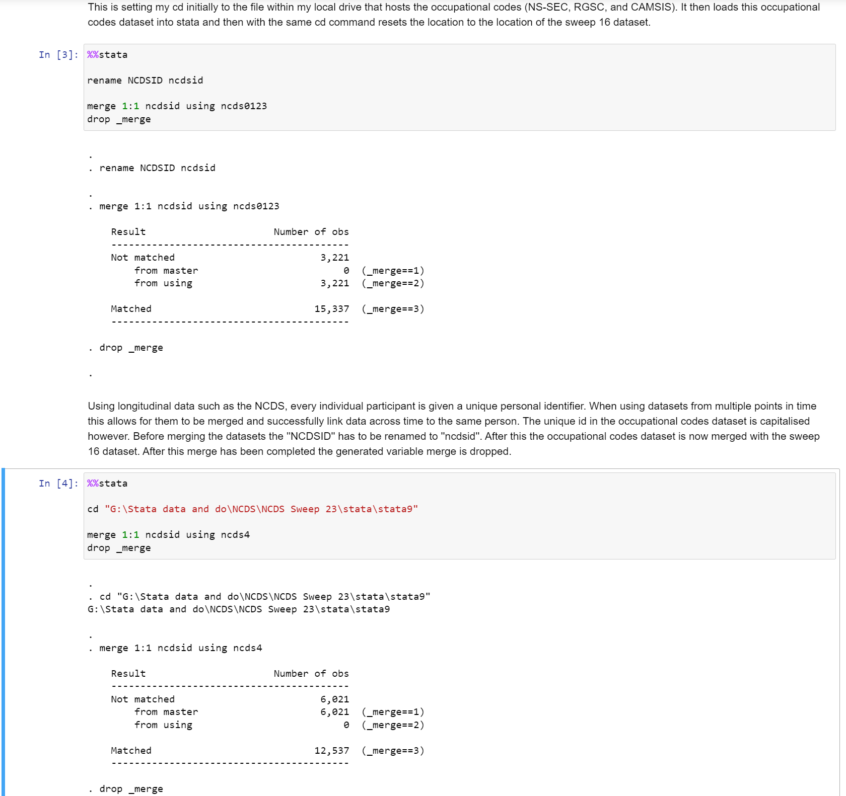
Through this process of combining code cells and Markdown cells, you know exactly what I am doing, and also exactly why I am doing it. These longer format ‘comments’ just don’t work properly in a .do file environment.
Keyboard Shortcuts:
One of the best tools that Jupyter has to offer is the ‘edit’ and ‘command’ modes. As a default when you are working away in your Notebook, you will almost always be in ‘edit’ mode - this can be seen by the cells being highlighted in green. If however you were to:
ctrl+enter
Whilst in an active cell, you will then enter ‘command mode’. Whilst in command mode the cells will turn blue and you will now have access to a whole host of keyboard shortcut commands that will make your life so much easier. Here is a general list of shortcuts that would be good to remember or keep handy as you are writing your Notebook - feel free to practice with them:
Toggle between edit and command mode with
EscandEnter, respectively.Once in command mode:
Scroll up and down your cells with your
UpandDownkeys.Press
AorBto insert a new cell above or below the active cell.Mwill transform the active cell to a Markdown cell.Ywill set the active cell to a code cell.D + D(Dtwice) will delete the active cell.Zwill undo cell deletion.Hold
Shiftand pressUporDownto select multiple cells at once. With multiple cells selected,Shift + Mwill merge your selection.1-6 will produce headers of different sizes to format your piece in a more professional manner
For the entirety of the keyboard shortcut options click on the keyboard icon at the top of the page.
More on Markdown
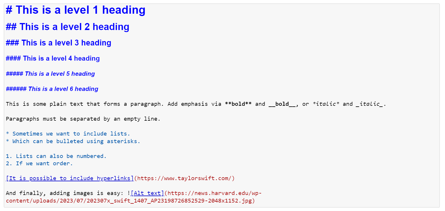
As mentioned previously Markdown cells are simple text editors - they work very similarly to any HTML enviroment. The basics of Markdown are very easy to master, but they do really enchance your Notebook and make it more comparable to a Journal Paper than a .do file. Here are the basics both written in editor mode in a Markdown cell:
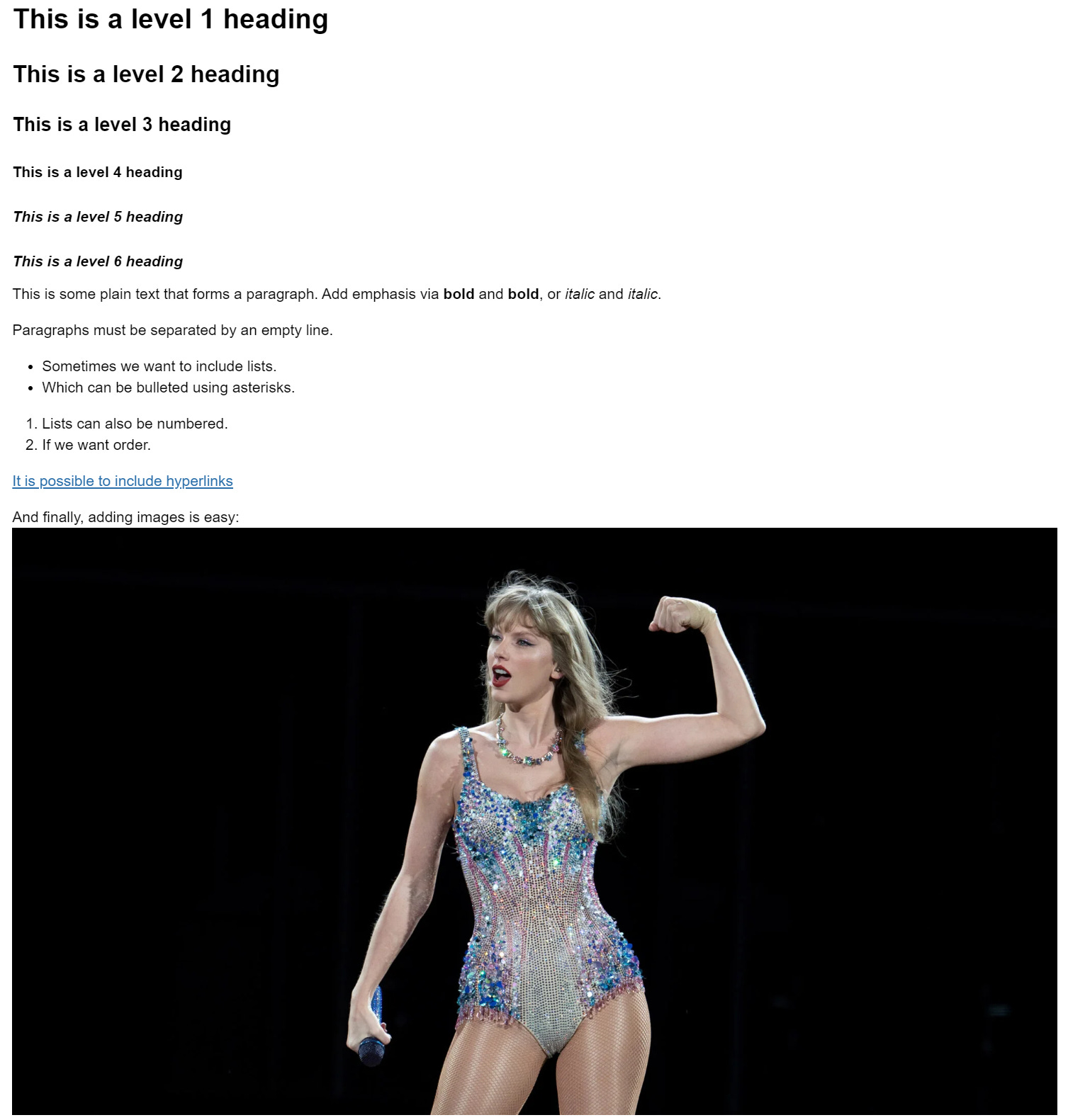
and also executed:
Jupyter Notebook can even be set up to produce equations as seen in Latex format within the same environment. This turns this Markdown comment:

Into this:

As a quick explanation of the syntax to be used in Markdown:
$ : All the Math you want to write in the markdown should be inside opening and closing $ symbol in order to be processed as Math
\beta : Creates the symbol beta
hat{} : A hat is covered over anything inside the curly braces of \hat{}. E.g. in \hat{Y} hat is created over Y and in \hat{\beta}_{0}, hat is shown over beta
_{} : Creates as subscript, anything inside the curly braces after _. E.g. \hat{\beta}_{0} will create beta with a hat and give it a subscript of 0
^{} : (Similar to subscript) Creates as superscript, anything inside the curly braces after ^
\sum : Creates the summation symbol
\limits _{} ^{} : Creates lower and upper limit for the \sum using the subscript and superscript notation
*** : Creates horizontal line
  : Creates space
\gamma : Creates gamma symbol
\displaystyle : Forces display mode (BONUS 3 above)
\frac{}{} : Creates fraction with two curly braces from numerator and denominator
<br> : Creates line breaks
\Bigg : Helps create parenthesis of big sizes
\partial : Creates partial derivatives symbol
\underset() : To write under a text. E.g. gamma under arg min, instead of a subscript
\in : Creates belongs to symbol
All set!
From here you now know the basics of Jupyter Notebook. You should be able to use Stata, write code, execute it, and create detailed well-formated text within one environment. For example, Jupyter Notebook demonstrates all the skills and tools that we have talked about up to this point check out a fantastic example of open science practices by Vernon Gayle and Roxanne Connelly. They have created a Jupyter Notebook for their entire research paper on “An investigation of Social Class Inequalities in General Cognitive Ability in Two British Birth Cohorts”.